From "Secondary Storage" To Just "Storage": A Tale of Lambdas, LZ4, and Garbage Collection

When we introduced Secondary Storage two years ago, it was a deliberate compromise between economy and performance. Compared to Honeycomb’s primary NVMe storage attached to dedicated servers, secondary storage let customers keep more data for less money. They could query over longer time ranges, but with a substantial performance penalty; queries which used secondary storage took many times longer to run than those which didn’t.

How come? We implemented secondary storage by gzipping data and shipping it off our servers' local storage onto S3. We also - crucially - did not spin up additional, expensive EC2 instances to handle the potentially vast amount of data involved in a secondary storage query. This often meant waiting for minutes rather than seconds, with larger queries sometimes timing out and failing entirely. It was a recipe for frustration, not least for us: prolific users of secondary storage ourselves.

Today things look very different. 20-minute queries are a thing of the past, and you may have noticed that the Fast Query Window indicator disappeared from the time selector. Queries which hit secondary storage are typically as fast as, or sometimes faster than, their all-primary-storage cousins. In this post, I'll explain how we got here.

Honeycomb query processing is fundamentally CPU-limited, and (for the most part) query time is a function of how much raw data needs to be read. Because we don't do any pre-aggregation, a one-week query means chewing up seven times as many bits as a one-day query, and so on. Secondary storage hugely expanded the amount of data we might have to examine, without adding a corresponding number of CPUs to the pool. Our work has focused on tackling both the compute efficiency of our code, and its ability to employ extra resources.

Supercomputing by the second

Honeycomb's storage servers spend most of their time relatively idle, ingesting data and waiting for their Big Moment when a customer query comes in. If the query is very large, what seemed like too many CPUs while idle suddenly isn't enough. Not nearly enough.

Enter AWS Lambda. Amazon's marketing of Lambda focuses on its use cases for data pipelines and as the basis of serverless API backends, but doesn't dwell on what the service actually is: CPUs on demand, sold in 100ms increments. It comes with significant limitations, but overcome these, and Lambda enables tremendous scalability in a sub-second timeframe.

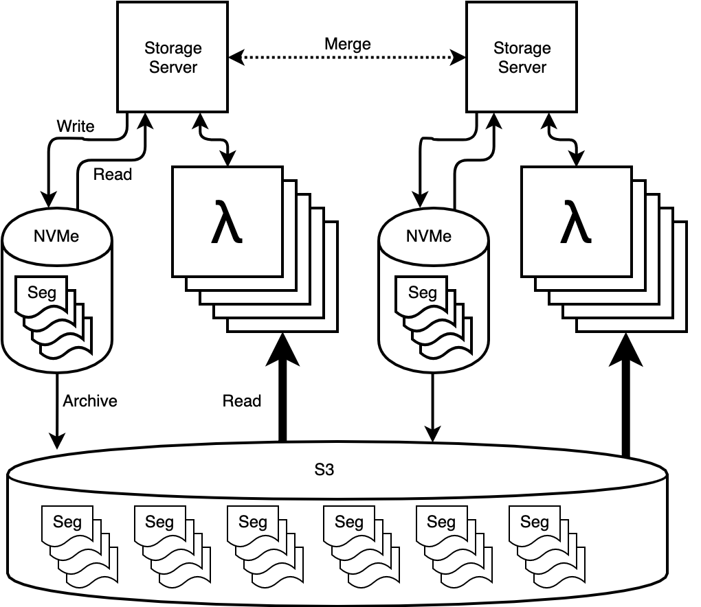
We use Lambda to accelerate the "secondary" part of secondary storage queries. For each segment (a roughly 1GB chunk of contiguous data), our servers call a Lambda function which pulls the data from S3, reads the necessary bits, and calculates its own local query result. This all happens concurrently, sometimes involving thousands of simultaneous Lambda jobs. Our servers then take the serialized responses and merge them together with the primary storage result. So, rather than acting as a server replacement, Lambda is effectively a force multiplier, with each of our own CPU cores overseeing the work of hundreds of others. When the query is done, all these extra resources disappear back into the cloud, to be summoned - and paid for - again only when needed.

The result is that querying over a lot of secondary storage data now needn't take much longer than querying over a little, something which would be cost-prohibitive to achieve without an on-demand compute service. For larger queries, this can be fully ten times faster, sometimes more.

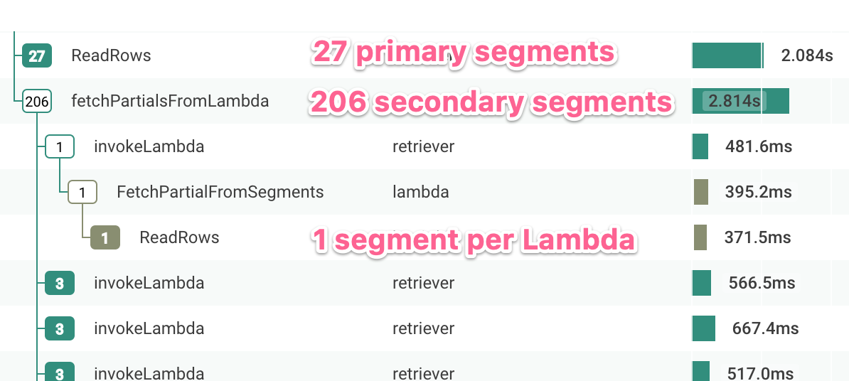
Part of a trace of a large secondary storage query using Lambda. Note: This is just one of many nodes involved in the query.

It's worth noting that Lambda CPU time is far more expensive than plain old EC2, so this model works best when demand is very bursty. For shorter-duration primary storage queries, which are the majority of our traffic, our servers are still doing the work locally.

Compression progression

Good old gzip. 27 years old, to be precise. Everybody uses it for something, and for us it was the default choice for compressing our secondary storage data. (We want to compress it for both economic and performance reasons; downloading smaller files is quicker.) But it turns out that in a world of high-bandwidth storage systems and network links, the CPU cost of decompressing gzipped data can outweigh the benefits. Today, there are superior alternatives for virtually any application.

And, it turns out, our original data format didn't compress well to begin with, especially given that we already use dictionaries for repetitious string columns. Designing a new compression-friendly file layout allowed us to switch from gzip to the speedy LZ4 without sacrificing much compression. It seems like a small thing, but the result was file reads around three times faster than the old gzipped format, and the speedup applied to all of our secondary storage data.

The war on garbage

Finally, we've done a lot of optimization over the past year, most of which follows a consistent pattern. (So consistent that I mentioned the same thing in last year's post about performance upgrades. The war continues.) If you've ever run pprof on a complex golang program, you've probably seen a box that looks like this:

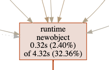
In non-garbage-collected languages such as C, heap allocation flows from an explicit source to an explicit drain. Allocate space with malloc() at the source, use it for a while, then release it into the drain with free(), and be very sure not to make a mistake with this or your whole day is ruined. Garbage collection frees us from the latter part of this equation; when you’re done with some scrap of data you can just sort of stop worrying about it. The runtime will take care of the rest. It's straightforward, and it works.

But it isn't free. For every pprof box like the one above, there's a similar box for the garbage collector. For Honeycomb's storage servers, it wasn't uncommon for allocation and cleanup to eat the bulk of CPU time, proportional to the size of the query. To make secondary storage work well, we had to reduce the flow from source to drain.

To do this, we had to go back to a more C-like model, and find the exact points where our most numerous heap-allocated structures expired, so that we could intercept them on the way to the drain. From there, rather than letting the garbage collector eat them, we could send them back to the source to be re-used. The exact flavor of this varies for each part of the data pipeline (sometimes we use sync.Pool, sometimes we don't), and in many cases involved modifying or removing particularly profligate third-party libraries. (Library authors: freshly-allocated heap shouldn't be the only possible way to get data out of your code and into mine.)

Together with more conventional code optimization and being careful to avoid spurious allocation, we’ve been able to roughly double the performance of the back-end portion of the query pipeline. As an added benefit, most of our servers’ CPU time is now spent doing actual work, which makes it much easier to understand profiles and reason about future improvements.

It adds up

Combine all of these improvements, and secondary storage queries look nothing like their long-running ancestors of last year. Especially thanks to Lambda, we’ve been able to simplify Honeycomb and remove the primary/secondary management headache. One less thing to worry about.

Want to find out just how fast Honeycomb queries are? Sign up for a free Honeycomb account today!