Virtualizing Our Storage Engine

Our storage engine, affectionately known as Retriever, has served us faithfully since the earliest days of Honeycomb. It’s a tool that writes data to disk and reads it back in a way that’s optimized for the time series-based queries our UI and API makes. Its architecture has remained mostly stable through some major shifts in the surrounding system it supports, notably including our 2021 implementation of a new data model for environments and services. As usage of this feature has grown, however, we’ve noticed Retriever creaking in novel ways, pushing us to reconsider a core architectural choice.

How does Retriever work?

Before I get into the nitty gritty of Retriever, I did want to point out that this is an internal change we made for performance—you don’t need to change the way you use Honeycomb at all!

Retriever is broken out into two distinct processes: 

• a writer, which receives a continuous stream of data and appends it to disk 
• a reader, which receives queries and uses data on disk to calculate aggregations and return results 

The writer is provided a stream of data in the form of “events,” which look like this:

dataset: rainbow_renderer
timestamp: 1714002225
-------------
error: "EOF"
duration_ms: 179
trace_id: 1156149343

Every event gets at least a dataset and a timestamp, along with an arbitrary set of additional keys and values (in the above example, an error message, a duration, and a trace ID). The reader process might then get a query like “quantity of EOF errors in rainbow_renderer over the past 7 days” and it will scan all the messages on disk where dataset = rainbow_renderer and error = EOF with a timestamp within the last seven days to calculate the answer. If you’re curious how our query engine works in more detail this talk from 2017 is still pretty accurate!

When the writer stores this data, it uses a directory structure that looks a bit like this:

├── rainbow_renderer
│   ├── segment1
│   │   ├── timestamp.int64
│   │   ├── error.varstring
│   │   ├── duration_ms.int64
│   │   └── trace_id.int64
│   └── segment2
│       ├── timestamp.int64
│       ├── error.varstring
│       ├── duration_ms.int64
│       └── trace_id.int64
├── goblin_gateway
│   ├── segment1
│   │   ├── timestamp.int64
│   │   ├── batch_size.float64
│   │   ├── db_call_count.int64
│   │   ├── trace_id.int64
│   │   └── slo_id.varstring

You’ll notice that the root contains a directory for each dataset (rainbow_renderer and goblin_gateway), each of which in turn contains subdirectories for something called a segment (segment1 and segment2). Within each segment, there are a bunch of files that actually contain event data: one file for each unique field. When we save a new event, we’ll append the data for each field to the appropriate file in the highest available segment. Our example event above would append to /rainbow_renderer/segment2/timestamp.int64, /rainbow_renderer/segment2/error.varstring, and so on.

On disk, the representation looks something like this:

# /rainbow_renderer/segment2/

timestamp.int64  error.varstring        duration_ms.int64   trace_id.int64
1714002221       ---                    ---                 2171666451
1714002224       ---                    1868                9462619034
1714002225       Error: unknown color   303                 2171666451
1714002225       EOF                    179                 1156149343

We group event data into segments as a way to limit the amount of data that needs to be read for each query. This allows us to make queries more efficient, as the most expensive thing that we do when we run queries is reading files from disk. So, if you’re looking for data from rainbow_renderer from the last 10 minutes, we might determine that you only need to read the files in segment2 because we stopped writing to segment1 30 minutes ago. However, for a longer query that looks over the past 60 minutes, we need to read the files in segment1 and segment2. This creates a dynamic where queries that look back over shorter periods of time tend to read less data from fewer files, making them more efficient.

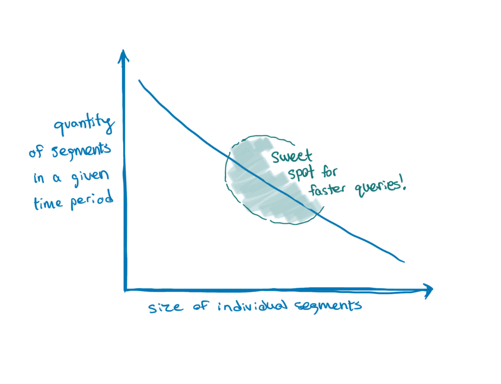
We automatically create new segment directories after every million events or every day (whichever comes first), so our chattier customers end up with more segments. This is beneficial for them because reading data takes time and often, we need to read data within segments from the beginning. We want to limit their size so we don’t end up spending extra time reading data from outside the query’s time range.

Out with the old, in with the new

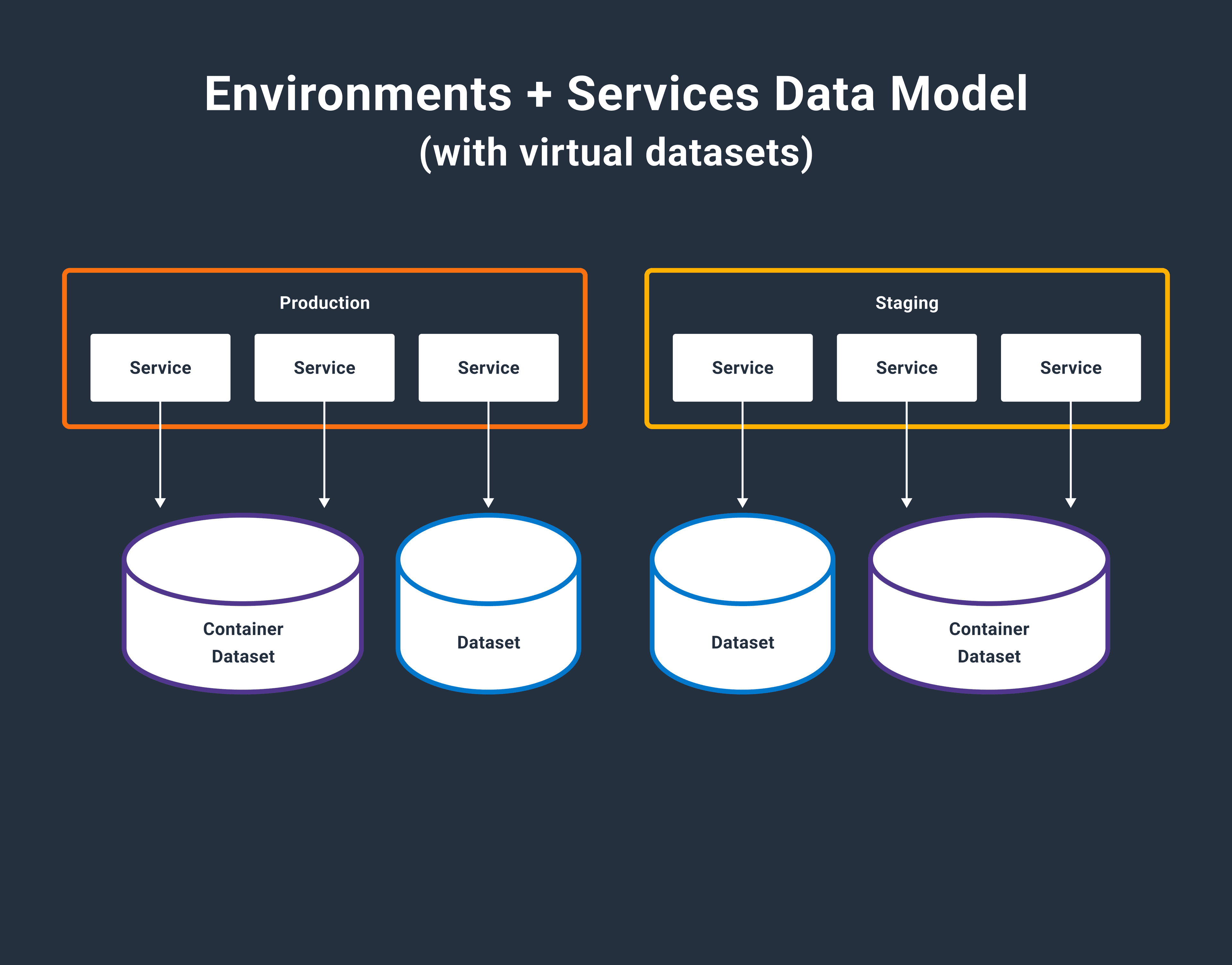
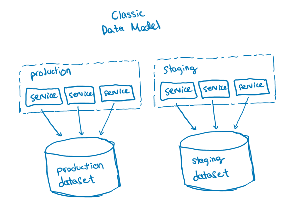
Prior to 2022, we encouraged our users to send all their data for a given environment into a single dataset so that they could query for data across all the services in an environment at once. This changed with the release of our new Environments and Services data model where environments became a first-class construct.

To support environment-wide queries in this new model, we gave Retriever the ability to query multiple datasets with a single query. A customer might, for example, want to view a trace in their system that has spans in two datasets: rainbow_renderer and goblin_gateway. Internally to Retriever, that query would end up needing to read files in /rainbow_renderer/segment2/ and /goblin_gateway/segment1/ to properly calculate its result. That’s not terribly different from the example above where we looked in multiple segments within the same dataset for results. The big distinction is that these two segments live in different datasets!

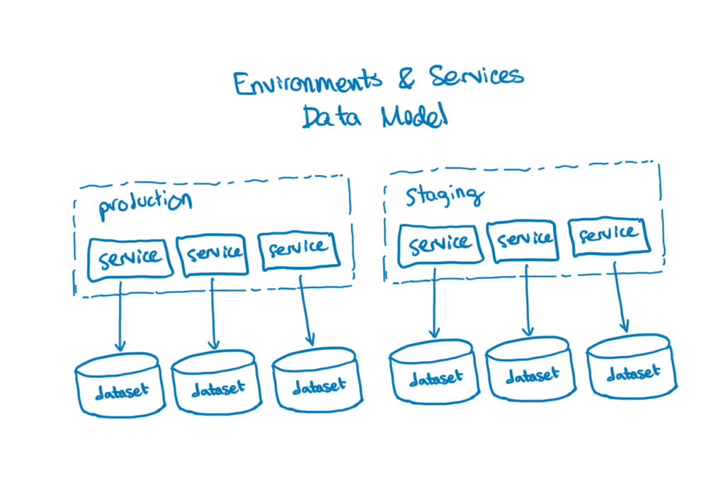
Aside from enabling this new data model, implementing multi-dataset queries resulted in a nice speed boost for single-service queries. Before E&S, most customers would send data from all their services to a single dataset—a single-service query in that world would need to read all the data for all the services in the time range, and filter out most of it to just read data for the relevant service. Now that each service lives in its own dataset, we didn’t need to do that filtering anymore, resulting in fewer segments to read and a higher likelihood that the data read was relevant to the query.

However…

On the other hand, queries that hit multiple services (like traces or relational queries) ended up needing to read more segments, resulting in slower queries. At the time, our bet was that customers would tend to scale up the number of events they sent us significantly more than the number of services their systems had, and with this assumption in mind, arranging our data this way seemed sensible.

As time went on and we grew, however, we started to onboard some bigger customers who had service-oriented architectures, sometimes with hundreds or even thousands of services. Because of the increased complexity of their systems, they had a greater need to run multi-dataset queries, and because they had so many services, we noticed that these queries were increasingly failing our internal query runtime SLIs due to time spent reading a growing number files from a growing number of segment directories. We needed a new strategy for arranging data on disk to support these customers and keep their queries running fast.

We needed to do this in a relatively focused way, without breaking the abstractions used by the rest of Honeycomb’s system, in which the “services” domain model was tightly coupled with our internal conception of “datasets.” We also wanted to do this in a way that minimized our need to rearrange existing data on disk, which would have been expensive and risky. After deliberation and planning, we ended up with a proposal we were proud of, which we called “virtual datasets.”

Our solution was to build a mapping layer between datasets-as-services (as understood by the rest of Honeycomb, and exposed externally) and datasets-as-filesystem-organization (as understood by Retriever, and opaque outside of the bounded context of our storage system). 

In this system, some services get combined together into “container datasets.” Other services can be kept as-is and left as “standalone datasets.” We are free to make these mapping decisions based on the ways we anticipate people might want to run queries, so that the most common queries read fewer files without needing to skip over irrelevant data.

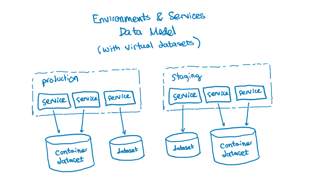
For example, if rainbow-renderer and goblin-gateway are services that often appear in the same traces and we find that a lot of the queries we run need data from both, we might combine the two services into a single container dataset, interleaving events from either service in the container. We keep track of which service each event is part of by maintaining a synthetic “virtual dataset” column. On disk, that looks a bit like this:

# /container_dataset_109872/segment4/

virtual_dataset.int64  timestamp.int64  error.varstring  batch_size.float64  (...etc)
<goblin-gateway.id>    1714002221       ---              32
<rainbow-renderer.id>  1714002224       EOF              ---
<rainbow-renderer.id>  1714002224       ---              ---

In this new virtualized world, we can run queries against both datasets by scanning the files as-is, and if we need to aggregate events specifically about goblin_gateway, our system will use records in the virtual_dataset.int64 file to filter out irrelevant events, in much the same way that it might use the error.varstring file to filter for events where error exists.

To maintain backwards compatibility as well as to allow us to modify these mappings over time, we maintain a historical log of when the mappings changed, and use it to determine which container datasets to look in for any given query. We’ve also built a system that uses metadata about event ingest volume along with specific heuristics about the data source to determine which mappings make the most sense. 

We intend to augment this system to use query history in order to tune these mappings based on anticipated future usage; we’re quite excited about where this system can go!

Significant improvements

After rolling out this change, we saw a significant improvement in query runtimes for bigger, more complex environments, including ones with more than 2,000 services and on the order of 100,000 events per second flowing into our system. Median query duration in situations like these started at around 20s (a customer experience we were certainly not proud of!) and decreased to around 0.2 seconds. That’s two orders of magnitude and well within our internal query performance SLOs. 

Additionally, this layer of abstraction affords us a lot more freedom to add more features to Honeycomb without worrying as much about the implications of our data model on query performance, since the two concepts are now (mostly) independent concerns. And finally, we’re brimming with ideas about how to leverage this new model to continue to improve query performance!

I’d love to hear your thoughts on where we could take this. Join us in Pollinators, our Slack community, to share your perspective.