Tracing OpenTelemetry

Infinite Retention with OpenTelemetry and Honeycomb

By Mike Terhar | Last modified on September 27, 2023

The needs of observability workloads can sometimes be orthogonal to the needs of compliance workloads. Honeycomb is designed for software developers to quickly fix problems in production, where reducing 100% data completeness to 99.99% is acceptable to receive immediate answers. Compliance and audit workloads require 100% data completeness over much longer (or "infinite") time spans, and are content to give up query performance in return.

Honeycomb has a 60-day retention window for your telemetry data. While there are a few ways to persist data indefinitely, in practice that means most of your telemetry data is gone after 60 days. While telemetry data older than 60 days isn't useful for a vast majority of organizations, some find themselves needing to retain their production telemetry for an indefinite amount of time. How do you store an infinite amount of telemetry for an infinite amount of time?

There are three ways to get infinite retention of trace data when using Honeycomb:

Query the data in Honeycomb: Honeycomb permanently stores the results

Look at a trace in Honeycomb: Honeycomb permanently stores the waterfall chart

Use OpenTelemetry to send traces to multiple locations: save the raw data in a persistent data store and pair that with a querying interface

This post will show you an experimental way to achieve the third approach using Amazon S3, Amazon Athena, and AWS Glue to build your own solution.

Should I create my own solution to this?

Your mileage may vary. A common use case for telemetry management pipelines is compliance and audit. Several commercial solutions exist like Cribl or ObservIQ, as well as open source solutions like OpenTelemetry.

If you decide to create your own long-term data retention and audit solution, you'll need to cobble together different components that can scale infinitely for the large volumes of data you'll inevitably generate.

The approach described in this blog results in a much slower data querying experience, so it’s unusable for real-time debugging in production. But it can meet rudimentary compliance needs and a proof-of-concept is shared here as a way to build a workable solution.

Permalinks in Honeycomb are forever

The first two infinite retention periods are for any query results that come from your data. The underlying data will age out in 60 days so that nice Raw Data tab won’t be able to help you anymore. The good news is that the chart and table data is enshrined into an object store that can be recalled forever. If you name your queries, you can find them with the search function. If you share the links in Slack or add them to an incident in Jeli, you can get back to them at any point in the future.

For trace waterfalls, the same is true. You can’t name the trace, but any links that are shared or saved will work long after the data has expired. Maybe other attributes are interesting a few months later? Good news: they’re still there!

OpenTelemetry S3 exporter

If you’re shipping data to your own S3 bucket, this isn’t really a Honeycomb retention change. It is a way to save these traces for as long as you may want. However, Honeycomb is good for urgency and breadth, so let’s use the right tool for the job.

The OpenTelemetry Collector has a delightful exporter, awss3exporter, that sends trace data directly to your own S3 buckets. You can create a data lifecycle that handles long-term storage. You can use Athena to query the S3 data, which is much less expensive since it doesn’t prioritize performance.

User experience comparison

This isn’t a way to get Honeycomb-like performance from S3. We are cobbling together some primitives with basic ClickOps user interfaces. No design effort went into this use case and it's pretty clear that this is something to tolerate rather than something to enjoy. There are also hidden costs and ways to accidentally owe Amazon a lot of money.

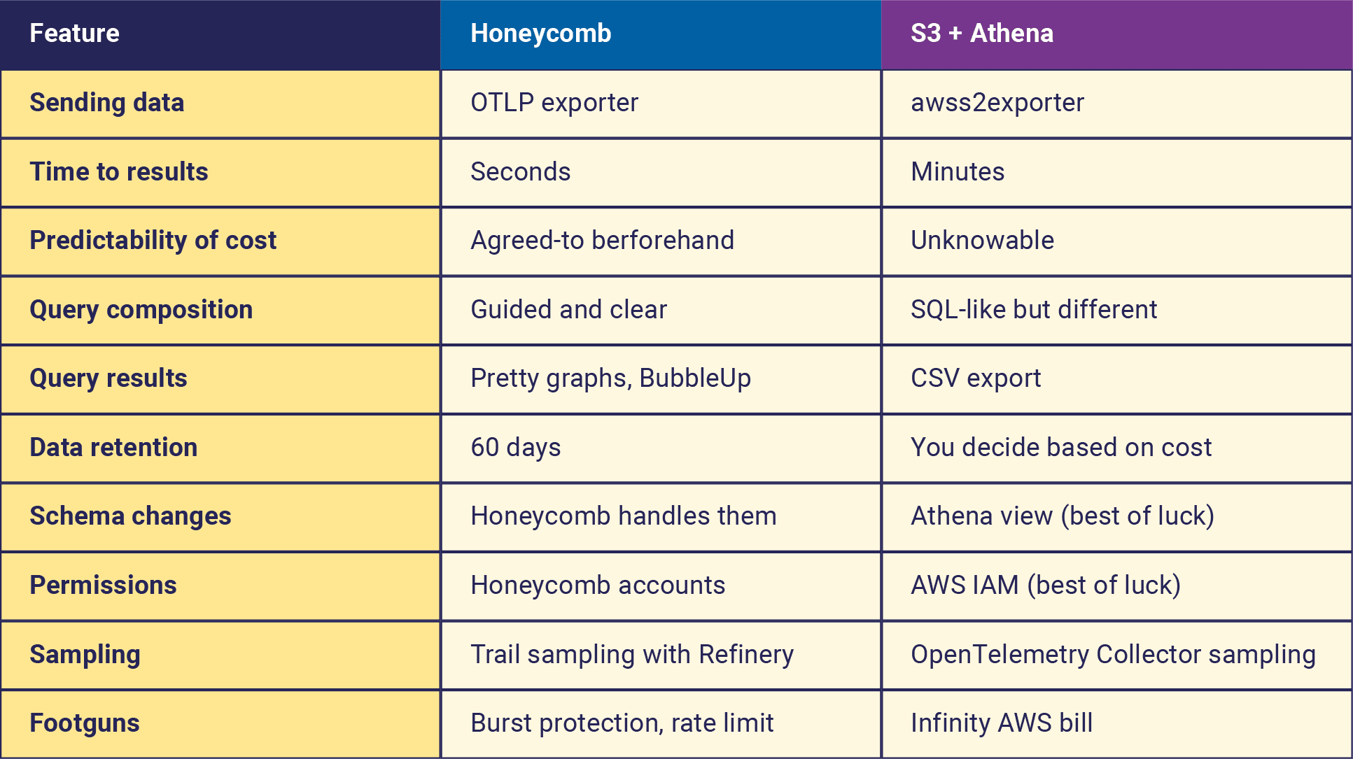
Infinite Retention: Comparing Honeycomb to Athena.

From the comparison here, we can see that Honeycomb is tuned for urgency and iteration, running many queries very quickly, at predictable prices, with visualizations that are comprehensible and intuitive.

There are many uses for telemetry beyond those that Honeycomb optimizes for:

Reviewing all sessions related to a specific IP address from some time ago

Evaluating specific span durations over long periods of time

Referencing very old data to compare performance year-over-year

The common thing about these is that it doesn’t matter how long the queries take or how annoying it is to process the data. These are pre-formed questions that may come from current events, but don’t impact the next step in your debugging adventure.

Architecture overview to add the exporter

Sending data to either Honeycomb or S3 is roughly the same amount of effort. You configure an exporter with credentials and the exporter delivers stuff in the right format.

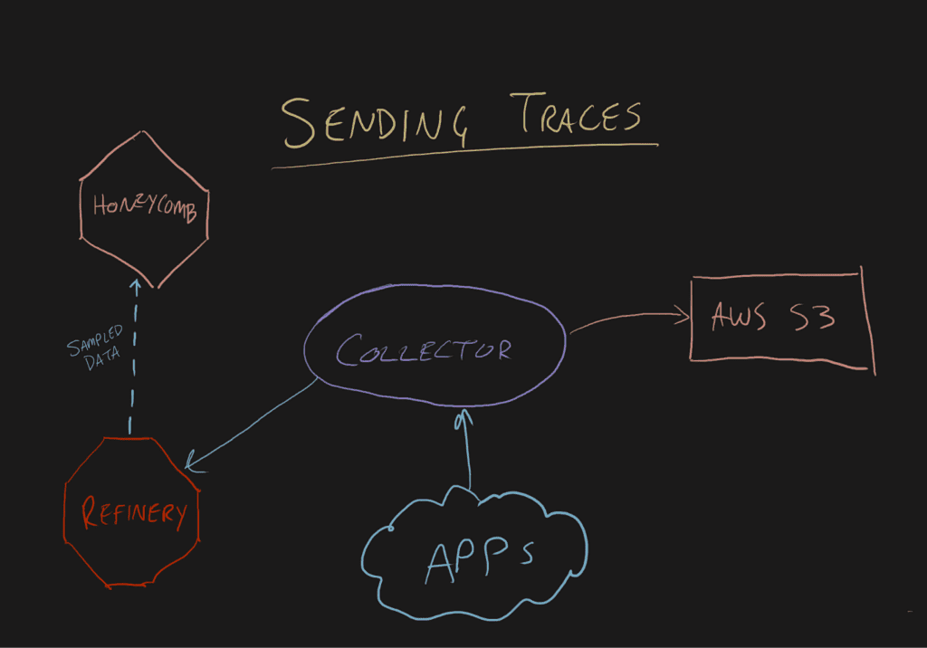
Infinite Retention: Diagram of sending traces to Honeycomb.

The one difference is that Refinery only emits Honeycomb-flavored data. If you’re using tail-based sampling, you’ll have an unsampled feed going to S3. This may be preferable, or it may be prohibitively expensive.

When it comes to querying, the differences are immense.

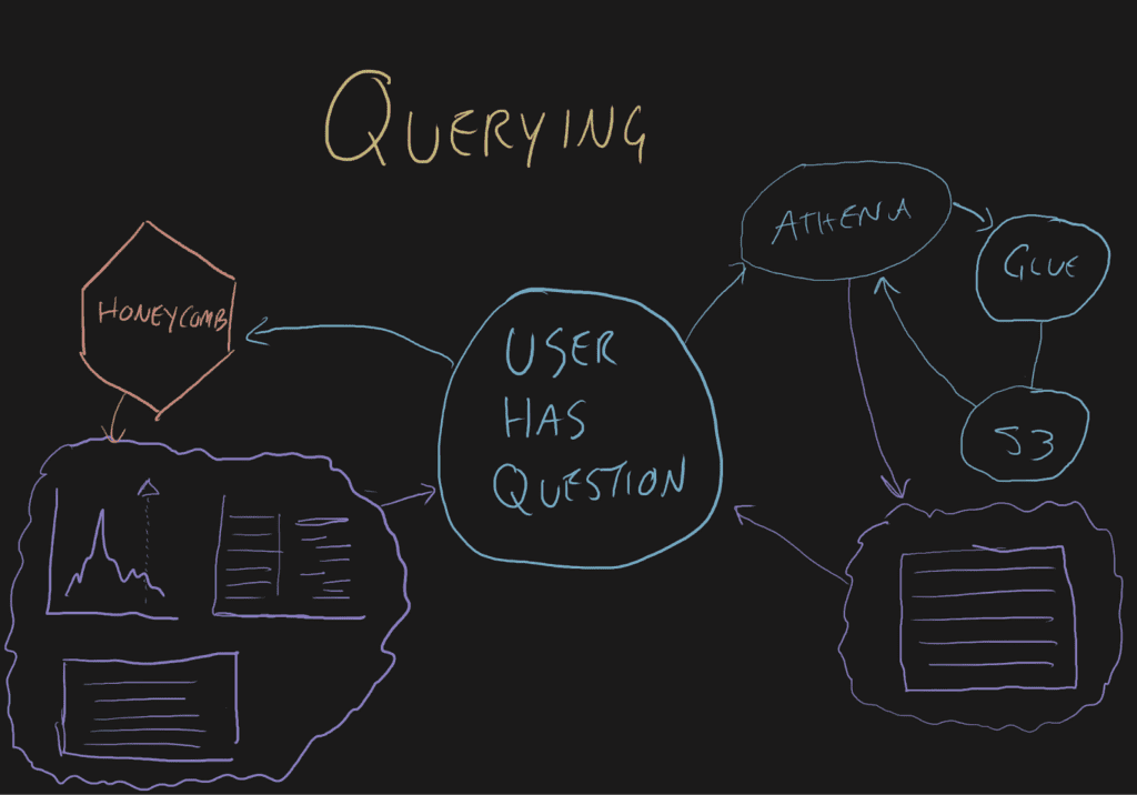
When a user has a question about something, they ask Honeycomb. Honeycomb gets the data, draws some visualizations or formats it into a Gantt chart and renders it for the human. Functionality like BubbleUp relies on the very flexible backend to compare hundreds of high-cardinality dimensions for you. The UI presents answers in a way that leads to the next query. And most importantly, each query with visualizations is presented in a few seconds so your mental model doesn’t have to be rebuilt between questions.

When a user asks something of Athena, they wait a while and then get a table that needs to be reassembled and run through another application for visualization.

Screenshots

How to achieve these amazing results for yourself

The summary of steps:

Create two AWS IAM roles, one for S3 writing, and one for Glue and Athena

Create two AWS S3 Buckets, one for trace data, and one for Athena results

Configure the awss3 exporter

Create a Glue crawler

Create an Athena view

Search and enjoy!

Create Amazon objects

1. Create an S3 bucket. I called mine `ca-otel-demo-telemetry`.

2. Create an S3-writable IAM account in AWS.

Make a new account with almost no permissions.

Policy example:

{
    "Version": "2012-10-17",
    "Statement": [
        {
            "Effect": "Allow",
            "Action": [
                "s3:PutObject"
            ],
            "Resource": [
                "arn:aws:s3:::ca-otel-demo-telemetry/*"
            ]
        }
    ]
}

If you’re in EKS, you can assign permissions to the pods using cloudy things. If you want to keep it simple for now, use the less secure access key approach.

Create an access key and export the variables into a name like TMP_AWS_ACCESS_KEY_ID and TMP_AWS_SECRET_ACCESS_KEY. If you don’t prefix them with TMP_ or something else, it’ll wreck your `kubectl` access.

Authorize the Collector to write to S3

In your Kubernetes cluster, at the Gateway Collector, add this code:

kubectl create secret generic aws-s3-creds --from-literal=AWS_ACCESS_KEY_ID=${TMP_AWS_ACCESS_KEY_ID} --from-literal=AWS_SECRET_ACCESS_KEY=${TMP_AWS_SECRET_ACCESS_KEY}

unset TMP_AWS_ACCESS_KEY_ID
unset TMP_AWS_SECRET_ACCESS_KEY

Then, you can check the secret with `kubectl get secret -n ca-otel-demo aws-s3-creds -o jsonpath='{.data}'`.

Configure the OpenTelemetry Collector

First, add environment variables to reference the access key and secret key from the secret we configured. The Collector Helm chart has a place to include environment variables, so you shouldn’t have to alter the chart or deployment.

If you have multiple Collectors in your telemetry pipeline, this should only be done at the Gateway since other Collectors enrich spans on the way to Honeycomb. You don’t want to miss any of that.

The other consideration is sampling. If you want to have an unsampled feed, be sure to use a separate pipeline or add this exporter at the load balancer:

env:
  - name: "AWS_ACCESS_KEY_ID"
    valueFrom:
      secretKeyRef:
        name: "aws-s3-creds"
        key: "AWS_ACCESS_KEY_ID"
  - name: "AWS_SECRET_ACCESS_KEY"
    valueFrom:
      secretKeyRef:
        name: "aws-s3-creds"
        key: "AWS_SECRET_ACCESS_KEY" 
[...]
config:
  exporters:
      awss3:
        s3uploader:
          region: 'us-east-2'
          s3_bucket: 'ca-otel-demo-telemetry'
          s3_prefix: 'traces'
          s3_partition: 'minute'

Finally, go into the pipelines that need to write to the S3 storage and add this exporter.

Now, deploy the OpenTelemetry Collector and see how things go! If it was already running, you may have to kill the pod to get it to accept the configuration changes.

Note for the future:

There is an emerging plan to add `encoding` options to exporters. Rather than using the default JSON marshaler to generate the text content that’s sent to S3, there may be friendlier formats available down the road. We’ll revise this POC once encoding options are available in the S3 exporter.

If the options exist in the future and you want to follow the approach as described below, the marshaler is called ptrace.JSONMarshaler from the go.opentelemetry.io/collector/pdata/ptrace module.

Check the S3 bucket for trace data

What you have now are very user-hostile JSON files in a deeply-nested S3 bucket tagging structure. I chose to break down the traces by minute, but you can pick your granularity depending on the volume of information you’re writing.

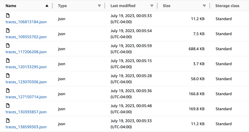
If data doesn’t show up, check the awss3 exporter repo for updates. It’s evolving software and may improve with breaking changes at any time.

Finding Answers

These JSON-formatted files in an S3 bucket are not very easy to find or deal with. AWS created two tools that help with this. One is Glue, which creates partitions for each S3 area and allows it to be queried by the other tool, Athena.

Glue converts the rough S3 files into a slightly less rough, but still pretty bad nested array.

In Athena, we create a view that sorts out the nested array into comprehensible rows.

Glue output:

Each row is an array derived from a JSON file which contains N resources that are mapped to M spans

Addressing the service.name field would look like: resourcespans[0].resource.attributes[0].value.stringvalue, but attributes[0] might not be always be service.name so you’ll have to try attributes[1] and attributes[2]—and maybe more, depending on the number of resources

Traces are mixed up across multiple rows and interwoven with unrelated spans

Sorting by time is limited to S3 directories

Athena view output:

Each row is a single span that has its associated resources, attributes, and events

Addressing service.name field is just `resources_kv[‘service.name’]`

Traces are found with clear where clause `traceId = ‘the trace id’`

Sorting by time can be done with nanosecond precision

Defining a schema with a Glue crawler

The OpenTelemetry schema doesn’t change when new attributes are added. Rather than using "attribute_key": "attribute_value" in a big array, the JSON output includes an array where it’s "attribute": { "key": "some_key", "value": { stringvalue: "some_string", intvalue: "some_int", etc }. This is nice for Athena because it means adding new attributes won’t change the schema. Upgrading to a new version of OpenTelemetry might.

Now that you have the short-term, high-quality, high-speed data in Honeycomb and an alternative storage in S3, let’s look at Athena to see how to query the data.

Create the database/columns using the AWS S3 Glue crawler with these instructions. It’ll ask if your data is already mapped. Say no. Use the S3 browser to find your bucket and traces directory.

Create another new IAM account for the crawler with a very limited policy.

Create a new database for ca-otel-traces with a low table limit. It should only need one called `traces`, but if you want to make different tables for different periods of time, give it a limit of one hundred.

Create the crawler, but don’t give it a schedule yet. In our OTel demo environment, it still takes about two minutes to run on an hour’s worth of data. About 12 minutes to run a day’s worth of data. A real production environment will likely be significantly busier with a lot more data.

Note: You must enable `Update all new and existing partitions with metadata from the table` or else the order of the items in the JSON changing will break the query.

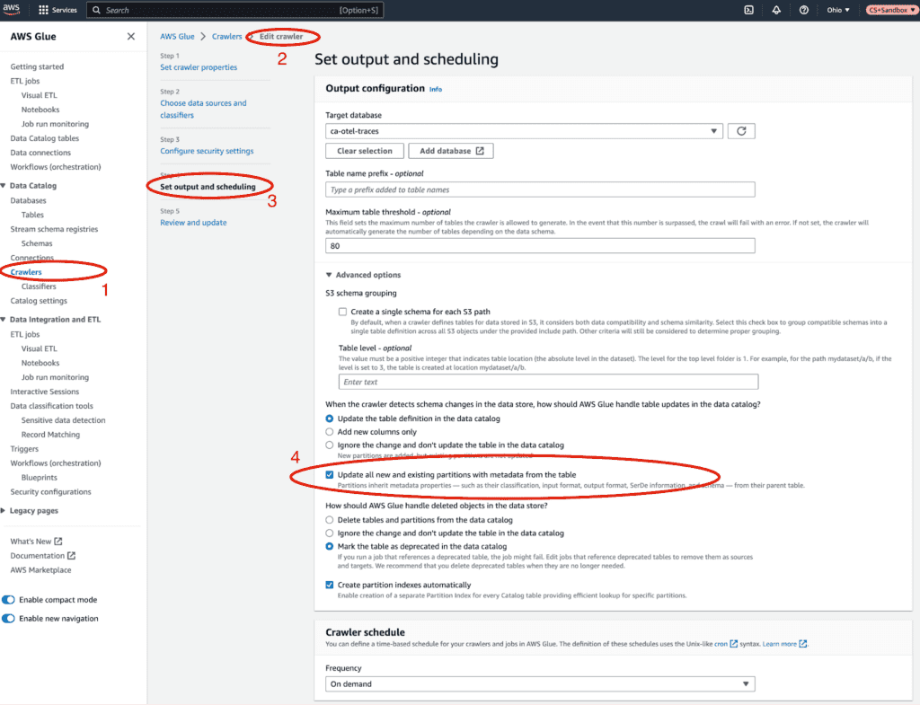
To run queries on the data, the Glue crawler needs to process it. This means if you expect people to run queries like this frequently, you can set the Glue crawler to crawl every day and just scan in the new items.

If you expect to never crawl this data until you need it, don’t create a Glue crawler for the whole traces folder. You can make specific month or day scoped crawlers that build smaller tables. This will increase the friction to query, but decrease the cost since it’s not creating all these extra partitions.

Review the thing Glue created:

{
  "resourcespans": [
    {
      "resource": {
        "attributes": [
          {
            "key": "string",
            "value": {
              "stringValue": "string",
              "arrayValue": {
                "values": [
                  {
                    "stringValue": "string"
                  }
                ]
              },
              "intValue": "string"
            }
          }
        ]
      },
      "scopeSpans": [
        {
          "scope": {
            "name": "string",
            "version": "string"
          },
          "spans": [
            {
              "traceId": "string",
              "spanId": "string",
              "parentSpanId": "string",
              "name": "string",
              "kind": "int",
              "startTimeUnixNano": "string",
              "endTimeUnixNano": "string",
              "attributes": [
                {
                  "key": "string",
                  "value": {
                    "stringValue": "string",
                    "intValue": "string",
                    "boolValue": "boolean",
                    "arrayValue": {
                      "values": [
                        {
                          "stringValue": "string"
                        }
                      ]
                    },
                    "doubleValue": "double"
                  }
                }
              ],
              "events": [
                {
                  "timeUnixNano": "string",
                  "name": "string",
                  "attributes": [
                    {
                      "key": "string",
                      "value": {
                        "stringValue": "string",
                        "intValue": "string"
                      }
                    }
                  ]
                }
              ],
              "status": {
                "message": "string",
                "code": "int"
              },
              "links": [
                {
                  "traceId": "string",
                  "spanId": "string"
                }
              ]
            }
          ]
        }
      ],
      "schemaUrl": "string"
    }
  ]
}

Now that we have a table, we can query it using Athena. If you run a query and it comes back empty, make sure the crawler created a partition for the year/month/day/hour combination that contains the data you want to find.

Setting up Athena

Make another S3 bucket for storing query results.

Athena will store search results in an S3 bucket, so we need to make one before we get to the settings page. I called mine `ca-otel-demo-athena-results`. Athena also points to a folder, so create a folder before navigating away. I made `results/`.

See the database in Athena:

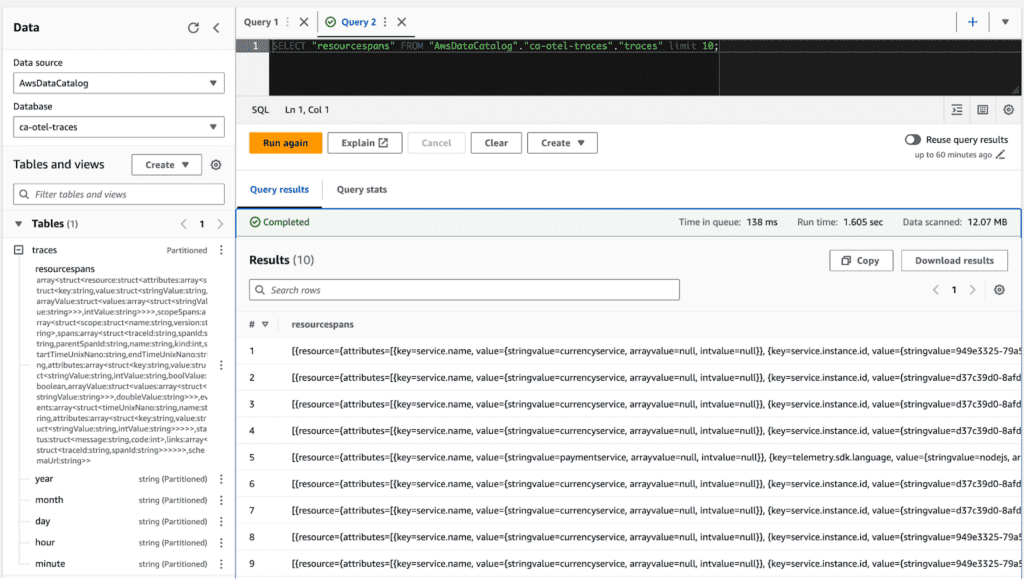
You’ll see the table on the left side with the big blob of fields under the `resourcespans` column, then the other partitions below.

Pull a few things using a query like below. Make sure the date and time numbers you’re using are among those that were crawled.

SELECT day, hour, minute, "resourcespans" FROM "AwsDataCatalog"."ca-otel-traces"."traces" 
where year = '2023' AND month = '07' AND day = '19' AND hour = '04'
order by day, hour, minute
limit 10

Notice that the statistics on the `Completed` bar show it’s going through quite a bit of work, even with only a couple of days of data.

Run time: 6.289 sec

Data scanned: 1.66 GB

But our output is an ugly nested array. To query a field within that array, we need to do a bit of unnesting and mapping.

Define Athena view to reference nested objects

If you want to get a list of service.name items present in that period of time, normally you’d make a query like `SELECT COUNT(*) WHERE year… GROUP BY service.name`. However, since service.name is in resourcespans[0].resource.attributes[0].value and it may move around to a different index thanks to JSON’s flexibility, we need to unnest and use a cross join to get access to the values in SQL.

Parts of the query

Athena uses mostly normal SQL keywords like SELECT, FROM, WHERE, ORDER BY, and LIMIT. I’m going to assume you’re familiar with those and focus on the weirder ones.

Unnest: Takes an array in a row and turns it into a bunch of rows with each item in the array turning into a key and some values.

Map_agg: Performs the opposite action of Unnest, but does so in a way that the “key value” becomes the key and the value array becomes a value.

Coalesce: Pulls each of the value objects and renders them as a string, which collapses the stringvalue, intvalue, boolvalue, and doublevalue into a string.

Intermediate table queries are used to perform each of the Unnest and Map_agg operations. There may be a way to perform all of these at once but I started this POC with no knowledge of Athena.

The big query to reassemble the nested array into flat, addressable maps

This query doesn’t scan data tables thanks to the first line. You can feel safe running this as long as it starts with `CREATE OR REPLACE VIEW`.

CREATE OR REPLACE VIEW "tracespansview" AS 
WITH resources AS (
		SELECT year,
			month,
			day,
			hour,
			minute,
			"$path" jsonfilepath,
			rss.resource.attributes r_attrs,
			rss.scopeSpans r_scopes
		FROM (
				"AwsDataCatalog"."ca-otel-traces"."traces"
				CROSS JOIN UNNEST(resourcespans) t (rss)
			)
	),
	resourceattrs AS (
		SELECT year,
			month,
			day,
			hour,
			minute,
			jsonfilepath,
			map_agg(
				s_attrs.key,
				COALESCE(
					s_attrs.value.stringvalue,
					s_attrs.value.intvalue
				)
			) resources_kv,
			s_scope.spans s_spans
		FROM (
				(
					resources
					CROSS JOIN UNNEST(r_attrs) t (s_attrs)
				)
				CROSS JOIN UNNEST(r_scopes) t (s_scope)
			)
		GROUP BY year,
			month,
			day,
			hour,
			minute,
			jsonfilepath,
			s_scope.spans
	),
	scopespans AS (
		SELECT year,
			month,
			day,
			hour,
			minute,
			jsonfilepath,
			resources_kv,
			span.traceId traceId,
			span.spanId spanId,
			span.parentSpanId parentSpanId,
			span.name spanName,
			span.startTimeUnixNano startTimestampNano,
			span.endTimeUnixNano endTimestampNano,
			span.attributes span_attrs,
			span.events span_events
		FROM (
				resourceattrs
				CROSS JOIN UNNEST(s_spans) t (span)
			)
	),
	spans AS (
		SELECT year,
			month,
			day,
			hour,
			minute,
			jsonfilepath,
			resources_kv,
			traceId,
			spanId,
			parentSpanId,
			spanName,
			startTimestampNano,
			endTimestampNano,
			map_agg(
				s_attrs.key,
				COALESCE(
					s_attrs.value.stringvalue,
					s_attrs.value.intvalue,
					CAST(s_attrs.value.boolvalue AS VARCHAR),
					s_attrs.value.doublevalue
				)
			) span_attr_kv,
			span_events
		FROM (
				scopespans
				CROSS JOIN UNNEST(span_attrs) t (s_attrs)
			)
		GROUP BY year,
			month,
			day,
			hour,
			minute,
			jsonfilepath,
			resources_kv,
			traceId,
			spanId,
			parentSpanId,
			spanName,
			startTimestampNano,
			endTimestampNano,
			span_events
	)
SELECT year,
	month,
	day,
	hour,
	minute,
	jsonfilepath,
	resources_kv,
	traceId,
	spanId,
	parentSpanId,
	spanName,
	startTimestampNano,
	endTimestampNano,
	span_attr_kv,
	span_events
FROM spans

If that query finishes successfully, you’ll see a new view pop into the left pane under Views. Now you can replace that query with a new, simple one as below.

Running queries

SELECT * 
FROM tracespansview
WHERE year = '2023' AND month = '07' AND day = '19' AND hour = '04'
	AND resources_kv['service.name'] = 'my_service'
LIMIT 1000;

Be sure to include year and month (and day, if possible) in the query so you only pull the S3 segments needed for the query to complete. If you don’t specify any of those or a limit, it’ll pull far too much data to be useful.

Example queries

The SQL nature of the interface allows for quality of life improvements to be made.

Duration_ms

SELECT traceid,
	spanid,
	spanname,
	starttimestampnano start_at,
	(
		cast("endtimestampnano" as BIGINT) - cast("starttimestampnano" as BIGINT)
	) / 1000 duration_ms
…

Since Glue treats everything as strings, we have to cast the nanosecond timestamps to bigints, then divide them by 1000 to get milliseconds. Not too difficult.

#	traceid	spanid	spanname	start_at	duration_ms
200	8c0e20546a49814233dd5bab37e87cdc	d6b9b1a580796cc2	grpc.oteldemo.CartService/AddItem	1689739184008000000	6395
199	f83e80a3ee6703f10f08275d1a2886d3	2953ecea18a948bb	HTTP POST	1689739184006000128	13316
197	5ed982d3ebc1e3370bbab17d70c12b21	19a1a2552ecd91c9	HTTP GET	1689739184004999936	4421
198	5ed982d3ebc1e3370bbab17d70c12b21	30157e966c457e59	grpc.oteldemo.CartService/GetCart	1689739184004999936	4251
196	5053d1f9831fa371de1d7eb06383c872	e0f77defd3ed45d6	HTTP GET	1689739184001999872	7020

Single trace

…
WHERE traceid = ‘trace id string’
…

The view presents `trace.trace_id` as `traceid`, so you can use it to filter.

Number of spans in each trace

SELECT COUNT(traceid) num_spans,
	traceid
FROM "ca-otel-traces"."spans2"
WHERE year = '2023'
	AND month = '07'
	AND day = '19'
	AND hour = '04'
GROUP BY traceID
LIMIT 1000;

#	num_spans	traceid
1	2	a6347e2440a37ec3655d222581c57da1
2	11	226d2f54cc8b3d50d327007b5547de95
3	20	37b6dfa7218c0aec275d2a62df0a69b3
4	3	b57c0e9a12a223c0a18bfc0c6ddd13bd
5	3	dd1476b0a4840c4a1fd888cc6e1a71aa
6	1	d61aba4a8b81a478d68d89168c940da3

Trace duration

SELECT min("starttimestampnano") first_span_start,
	max("endtimestampnano") last_span_end,
	(
		cast(min("endtimestampnano") as bigint) - cast(min("starttimestampnano") as bigint)
	) / 1000 as total_duration_ms,
	traceid
FROM "ca-otel-traces"."spans2"
WHERE year = '2023'
	AND month = '07'
	AND day = '19'
	AND hour = '04'
GROUP BY traceID
LIMIT 1000;

#	first_span_start	last_span_end	total_duration_ms	traceid
1	1689740334211694681	1689740334252999501	41304	5e7ac20a2acfecb7694f667d8c044745
2	1689742239635550055	1689742239662938363	25612	0675d48798e26658a5764a77cc58afe3
3	1689740637508000000	1689740637581031936	43372	64c5e18613da213f6a4e203a517c8a51
4	1689742298423000064	1689742298469735127	24369	39a9f4f0762034024b46a009592240c8
5	1689742140724999936	1689742140733933568	1592	f0e22194df92f7250af7dc4b935e5c8c

Saved queries

If you find a query useful, you can use the hamburger menu at the top of the query editor to save the query and give it a name.

Query history

After running a few example queries, you can go over to the `Recent queries` tab and see some that ran previously.

Multiple tables from smaller Glue runs

If you create new tables for different Glue runs to limit ongoing cost, create multiple views of those tables. In the huge view query above, you’ll see `FROM "AwsDataCatalog"."ca-otel-traces"."traces"` which is the table I have Glue scrape all my traces into. You may want to create tables like `traces_202307` and index July into that table.

Conclusion

You now have a backup plan. If something goes awry and you need something from 62 days ago, you can get to it without a time machine.

This is a rough POC. If you have experience or opinions on ways to improve this, I’d love to hear from you in our Pollinators Slack in the #discuss-aws channel.

OpenTelemetry Observability